Risk and Return Concepts
Readings: Chapter 5
At the end of this unit students should be
able to:
-
Define dollar return and rate of return.
-
Define risk and calculate the expected rate of return,
average rate of return, standard deviation, and coefficient of variation for
a probability distribution.
-
Specify how risk aversion influences required rates of
return.
-
Graph diversifiable risk and market risk; explain which
of these is relevant to a well-diversified investor.
-
Explain how and why a portfolio’s risk may be reduced.
-
State the basic proposition of the Capital Asset
Pricing Model (CAPM).
-
Explain the significance of a stock’s beta
coefficient, and use the Security Market Line to calculate a stock’s
required rate of return.
-
List changes in the market or within a firm that would
cause the required rate of return on the firm’s stock to change.
- Identify concerns about beta and the CAPM.
| Definitions
and Computations
|
|
As was
mentioned in our introductory lecture, a factor which affects the goal of
shareholders' wealth maximization is the element of risk.
Risk
reflects the uncertainty surrounding the outcome of future events. In the case
of a security, a risky security is one in which the expected outcome
(pay-off/return) may be different from the actual outcome. The greater the
difference, the more risky the security.
|
| Measuring
Risk
|
| Researchers
have developed the use of the term, standard
deviation to measure risk (This risk element as measured by the
standard deviation is also known as 'stand alone' or 'total' risk, and refers to
the risk inherent in an investment/asset if that investment/asset were
held in isolation). Now once we speak about future events, of which we are never certain, we have to incorporate
the likelihood of the outcomes materializing. This likelihood is accounted for
by the use of probabilities. However, before we evaluate the riskiness of an
expected outcome we need to first determine the expected outcome/return itself.
|
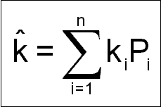
| Expected
Return or Mean:
|

|
| Note
-
the result obtained will be in the same denomination as the individual returns
(i.e. $ then $ or % then %)
|
| Where P
= the probability of state i occurring
and k = the expected return if state i
occurs and n = the number of different states of occurrences..
|
|
| Having
determined the expected return, we can now find the standard deviation, which is
given by
:

|
|
|
|
Note -
the result obtained will also be in the same denomination as the individual
returns (i.e. $ then $ or % then %)
|
|
|
| Illustration 1 |
|
Stock A
may provide you with the following returns based on the state of nature
that exists:
State
of Nature
Probability of state occurring
Return
Boom 0.20
70%
Stagnation
0.50
30%
Recession
0.30
-10%
|
|
The expected return is:
| 0.2 |
x |
70 |
= |
14 |
|
| 0.5 |
x |
30 |
= |
15 |
|
| 0.3 |
x |
-10 |
= |
-3 |
|
|
|
|
= |
26 |
% |
|
The standard deviation is:
|
- This
stock has an expected return of 26% and a standard deviation of 28%.
|
| Illustration 2
Stock B
may provide you with the following returns based on the state of nature
that exists:
State
of Nature
Probability of state occurring
Return
Boom 0.30
21%
Stagnation
0.40
11%
Recession
0.30
-2% |
The expected return is:
| 0.3 |
x |
21 |
= |
6.3 |
|
| 0.4 |
x |
11 |
= |
4.4 |
|
| 0.3 |
x |
-2 |
= |
-0.6 |
|
|
|
|
= |
10.1 |
% |
|
The standard deviation is:
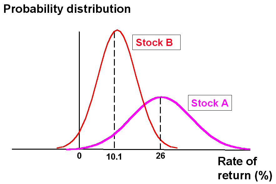
Because
of the smaller range of variability, Stock B is less risky as illustrated below
in the graph:
Graph 4.1
 .
.
Which stock is the preferred option?
The
preferred option depends on your attitude towards risk: If you are risk
averse,
then you hate risk and initially may decide to choose option 2. If you love risk
you may decide to choose option A, because of the higher expected return.
However, as in this situation, once the expected returns are different for each
option, a more scientific approach to determining the better option is to
calculate what is called the "Coefficient of Variation (CV)"
This
is found by the formula:
|
|
| CV = |
Standard Deviation |
|
Mean |
|
The
result which is expressed in absolute terms, gives a figure which expresses the
amount of risk involved per unit of
return.
For
Stock A,
For
Stock B,
In
finance this is the preferred approach, hence Stock B is better as it provides
only 0.891% of risk for every 1% of return as opposed to Stock A which is 1.077%
of risk for every 1% of return.
Note, in reference to the
last point - As it relates to the usage of the CV, always compute it to decide
upon investments if a decision cannot be based solely upon returns or upon
standard deviations. In other words we assume in finance that every individual
is risk averse.
Risk
aversion and rates of returns
As just mentioned above, an
individual who is risk averse hates risk. Consequently, he or she will demand a
greater rate of return for a risky investment to compensate themselves for this
risk element. Therefore, in summary, riskier investments will attract greater
rate of returns.
Realized
returns/historical data
In
our previous discussion we looked at future events. It is common for historical
data to be used to analyze the return and riskiness involved with a
particular investment.
Illustration 3
Stock C
had the following prices and issued the following dividends throughout the
last 6 months:
Month
Price $
Dividends $
Jan
13.75 -
Feb
15.25 3.00
Mar
17.85 1.00
Apr
16.50 -
May
15.00 4.00
Jun
18.05 2.00
A
shareholder bought this stock in January for $13.75
If
we recall from the introductory lecture, the wealth of a shareholder is
effectively improved if the price of each of his shares increases. It is also
improved if he received any dividends. We can always quantify this improvement by
calculating his return for the periods in which he held this share. Using the
illustration, his return for the period Jan-Feb can be computed using the
following two steps;
(a)
computing his capital gains yield (change in price)
| 15.25 - 13.75 |
= 0.1091 |
= 10.91% |
| 13.75 |
|
|
|
(b)
computing his dividend yield (his cash inflow as % of the original
price)
| 3.00 |
= 0.218 |
= 21.8% |
| 13.75 |
|
|
|
The
sum of these two will give his total yield/return
for the period:
In
general the holding period return for any security for time t can be found by the following
formula:
| Pt -
Pt-1 |
|
Cft |
|
Pt -
Pt-1 + Cft |
| ----------------- |
+ |
---------------- |
= |
---------------------- |
| Pt-1 |
|
Pt-1 |
|
Pt-1 |
| Capital
gains yield |
|
Dividend
yield |
|
|
|
Let's
complete the other periods:
Feb-Mar:
| 17.85 - 15.25 + 1.00
= |
3.6 |
= 0.2360 |
= 23.6% |
| 15.25 |
15.25 |
|
|
|
Mar-Apr:
| 16.50 - 17.85 + 0 = |
-1.35 |
= - 0.0756 |
= -7.56% |
| 17.85 |
17.85 |
|
|
|
Apr-May:
| 15.00 - 16.50 + 4 = |
2.5 |
= 0.1515 |
= 15.15% |
| 16.50 |
16.50 |
|
|
|
May
- Jun:
| 18.05 - 15.00 + 2 = |
5.05 |
= 0.33666 |
= 33.67% |
| 15.00 |
15.00 |
|
|
|
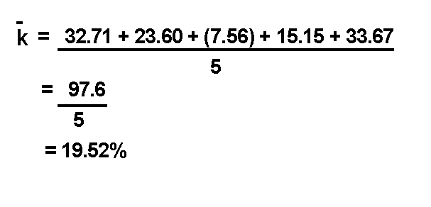
We
now have the returns for the five periods. We can now calculate the shareholder's
average return for the 6-month period.
Note - we use the term average because the returns have already taken
place (as opposed to expected).
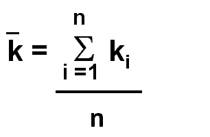
Average
Return: (Note the change in the formula)
Therefore
the average return is :
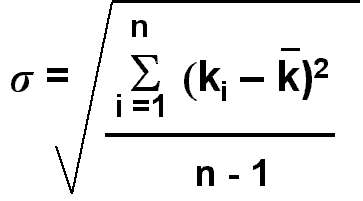
To
determine the standard deviation we must note that - the formula changes as well
Standard deviation:
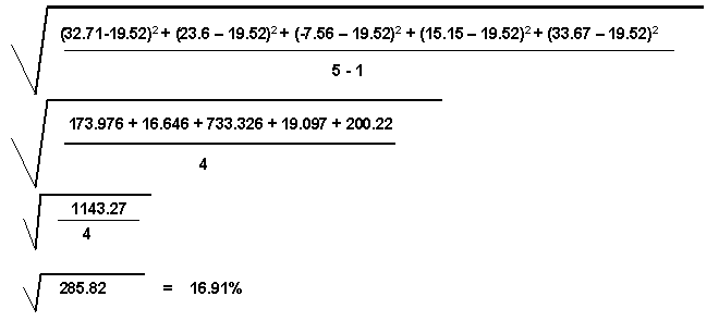
Therefore
the standard deviation is:
The
formula for the CV remains the same, therefore the CV is:
|
|
|
| CV = |
16.91% |
= 0.866 |
|
19.52% |
|
|
Therefore the stock provided
0.87% risk per 1% of return.
Portfolio Risk
Broadly
speaking risks in Finance can be classified into three types of risks - Business
Risk, Financial Risk and Portfolio Risk
Business
Risk refers to the uncertainty a company has with regard to its operating
income.
Financial
Risk refers to the extent to which
a company is financed by debt and the volatility of its net income caused by the
corresponding interest expenses .
Our
focus, however will be on Portfolio Risk.
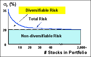
As previously mentioned, risk that is estimated by the standard
deviation is known as 'stand alone' or 'total risk' which is comprised of
(1)
Non-diversifiable risk/ market risk/ systematic risk
(2)
Diversifiable risk/firm-unique risk/company specific risk/un-systematic
risk
Non-diversifiable risk - is that quantity of
risk which cannot be diversified away by combining assets into portfolios. It
results from general macro-economic factors such as inflation, interest rates,
war etc.
Diversifiable risk is that component of risk
which results from factors which are unique to the individual firm e.g. the type
of product it produces, the industry it is in or the level of gearing (amount
debt in its capital structure). This type of risk can be reduced or totally
removed by appropriately combining individual assets with other assets in a
portfolio. So then, diversification is the process whereby individual assets are
combined with each other in a portfolio in an attempt to increase returns
without a commensurate increase in risks.
Graph 4.2:
The
reduction of portfolio risk by diversification is only possible if assets which
are not perfectly positively correlated
with the existing portfolio are added.
Correlation
Correlation
in this context refers to the degree to which one asset moves with another
asset. Correlation between two assets is measured by what is called the
correlation coefficient, 'r'.
The values for 'r'
ranges from +1
to -1 .
|
+1
=> two assets are perfectly positively correlated
-1
=> two assets are perfectly negatively correlated
0
=> two assets are not correlated, i.e. they move
independent of each other
|
The ideal objective of diversification of a portfolio is to add assets which are
perfectly negatively correlated to the existing assets in the portfolio.
Therefore,
decreases in the returns of some will be offset by increases in the returns of
others. In reality, one never finds assets which are perfectly negatively
correlated, however the closer the correlation coefficient is to -1, then the
more the portfolio risk will be reduced.
Expected
Return and standard deviation of a portfolio
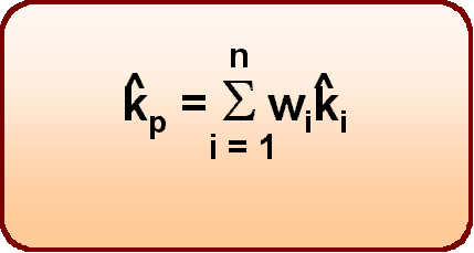
For a n-asset
portfolio, the expected return is given by:
Where wi
is the weight of asset i. (That is, the proportion of funds
invested in asset i)
For a 2-asset portfolio (stocks a and b),
the standard deviation is given by:
Where rab is the correlation coefficient
between stocks a and b.
Note - as mentioned, this is the standard
deviation formula for a 2-asset portfolio. The formula for a portfolio
which exceeds 2 assets is extremely complex and will not be explored.
However, the formula for the expected return applies to any number of assets in the
portfolio.
Illustration
4
A
company is considering two stocks A and B, in which it will invest 60% and 40%
of funds available, respectively. The correlation coefficient is -0.7 and other
related information is presented below:
Stock A
Stock B
Expected
Return
10%
12%
Standard
deviation
2%
4%
Coefficient
of variation
0.2
0.33
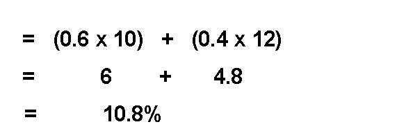
The
expected return is :
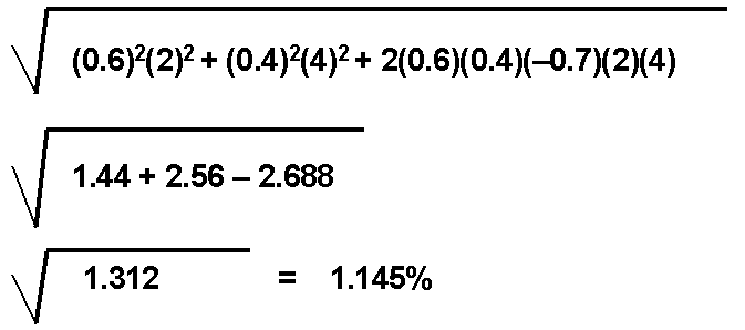
The
standard deviation is:
The
coefficient of variation is:
|
| CVp = |
1.145% |
= 0.106 |
|
10.8% |
|
|
Analysis:
The expected return of the portfolio is greater than that of stock A
although it is lower than that of stock B. The risk ( as per the standard
deviation) of the portfolio is lower
than either of the two stocks. The question is now this...Is stock B preferred to the portfolio of stocks A and B? The answer rests with the CV. The
portfolio has the lower CV, hence it is the preferred investment.
Capital
Asset Pricing Model(CAPM)
It
is always assumed that the more risky assets are, then the greater the return
should be to compensate for this risk. But how does one know what level of
return that is appropriate for a given level of risk?
In
answering this question, the model (CAPM) was developed with the aim of finding
the required return on an asset given
a particular risk element contained in it. This particular risk element is Beta
(b)
which measures the level of riskiness of the returns of the asset/security with
respect to that of the market. In other words, Beta shows how risky a
stock is if the stock is held in a well-diversified portfolio
.In
essence then, b
measures non-diversifiable risk i.e. market risk.
(Note - if the stock is not held in a well diversified portfolio then
beta is not relevant, but stand-alone risk is.)
As
previously mentioned the rate of return of an asset is equal to a risk-free
portion plus a risk premium. The CAPM formula expresses this relationship in a
similar manner as follows:
Where:
ks = the required return of the security
krf = the nominal risk free rate
km = the average return on the market
bs
= Beta of the security
Also
note that:
(km - krf)bs
= the
risk premium
(km
- krf)
= the market premium, i.e. the premium that the market provides over the risk
free rate
A
security with a beta of 1 indicates that the security is equally as risky as the
market. It also indicates that the scrutiny is similar to the average security
on the market and thus will have a return similar to that of the market return.
This
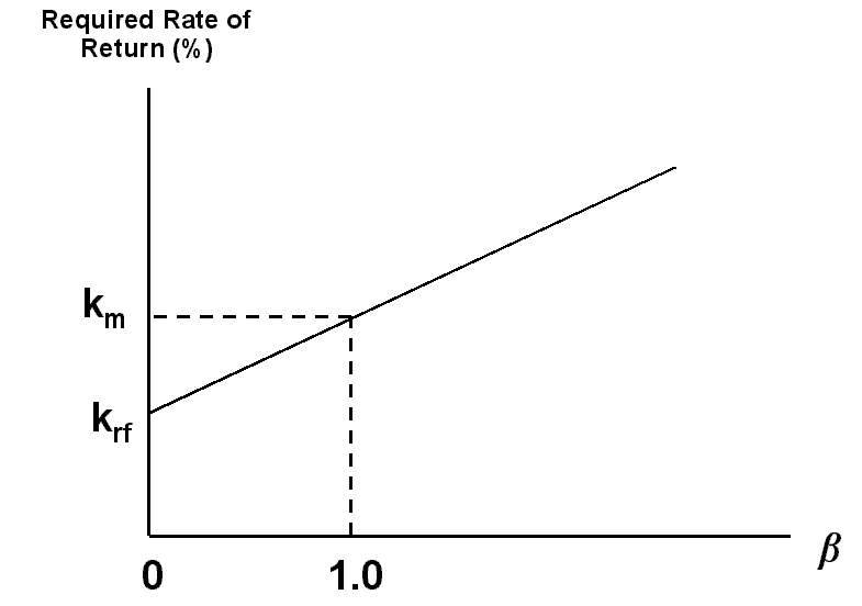
can be seen by placing b=1
into the equation:
|
ks =
krf + (km –
krf)bs
ks =
krf + (km –
krf)1 ks =
krf + km –
krf
ks =
km
|
A
security with a beta of 0 indicates that the security is risk-less. It also
indicates that the scrutiny moves independent of the market and thus will have a
return similar to that of the risk free return. When we place b=0
into the equation we see:
|
ks =
krf + (km –
krf)bs
ks =
krf + (km –
krf)0
ks =
krf
|
However,
a beta of 2 indicates that the security is twice as volatile as the market but
it does not mean that the required rate of return of this security will be twice
that of the market.
The
graph of the CAPM known as the Security Market Line (SML): Graph 4.3: (This
graph shows the relationship between an asset's required rate of return and its
beta.)
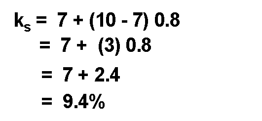
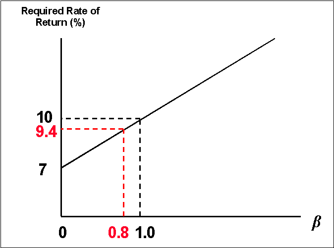
Illustration 5
If
the treasury bill rate is 7% and the return on the market is 10%, then what is
the required rate of return on a security whose beta is 0.8?
Draw the SML, and label accordingly.
Solution:
Graph
4.4:
Factors
that cause the required rate of return of a stock to change
As
previously mentioned the SML shows the required rate of return of a particular
asset given its Beta. Generally, the required rate of return of an asset is
equal to its expected rate of return, in which case the asset is said to be in
equilibrium. However, there may be occasions when the required rate of return
will change and therefore will not equal to the expected rate of return. The
factors that would lead to such a change are:
-
Changes
in inflation which would lead to changes in the risk-free rate.
-
Changes
in external factors and a company's financial structure which would lead to
changes in beta.
-
Changes
in an investor's risk aversion which would lead to changes in the market
premium.
Incorrectly priced assets
(those not in equilibrium)
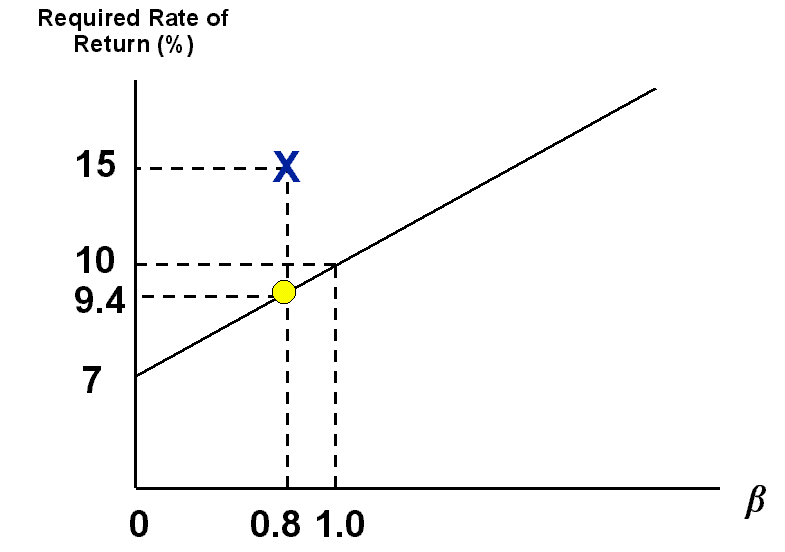
Looking
at the previous example, let's assume that the security had an expected return
of 15%. Its position on the SML would be as follows:
Graph
4.5:
Here
the expected return > the required return i.e. the expected return is above
the SML. "What does this mean?"
The
required return is only 9.4% but it
is expected to have a return of 15%,
therefore the asset is worth purchasing.
An
alternate analysis is that assets which have high returns are usually very risky
and consequently lowly priced, as in this case. By extension, this asset would
be priced at an amount lower than it should really be (undervalued). It is therefore an
attractive asset to purchase.
Note
- The converse also holds, i.e. if the expected return falls below the SML
=>highly priced/over priced
SML for a portfolio
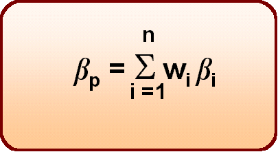
A
SML can also be constructed for a portfolio of stocks, using the same CAPM
equation. However, we would need to determine the beta of the portfolio,
which is given by the formula::
where
bi
is the beta of stock i.
Concerns
about beta and the CAPM [1]
The
CAPM is more than just an abstract theory described in textbooks - it is also
widely used by analysts, investors, and corporations. However, despite the
CAPM's intuitive appeal, a number of recent studies have raised concerns about
its validity. In particular, a recent study by Eugene Fama of the University of
Chicago and Kenneth French of Yale found no historical relationship
between stocks' returns and their market betas, confirming a position long held
by a number of professors and stock market analysts.
If
beta does not determine returns, what does? Fama and French found two variables
that are consistently related to sock returns: (1) the firm's size and (2) its
market/book ratio. After adjusting for other factors, they found that smaller
firms have provided relatively high returns, and that returns are higher on
stocks with low market/book value ratios. By contrast, they found no
relationship between a stock's beta and its return.
[1]This section has been taken directly from the text, page 204 ( the first two paragraphs of the section with the same heading)
